Note

Click here to download the full example code

The "Dual Mass Oscillator"

This example demonstrates how to use CoFMPy to run the well-known Dual Mass Oscillator example. The system simulates two masses connected with three springs and dampers on two walls.

The system is composed of two FMUs that are connected together. After describing the FMUs and the connections between them, we will run the simulation and plot the results.

The FMUs are provided by OpenModelica and are available in the OMSimulator Github repo.

Warning

The FMUs are currently not working on Windows OS. We recommend using a Linux system to run this example.

Description of the system

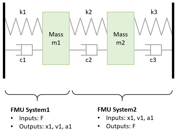
The Dual Mass Oscillator is a mechanical system composed of two masses, each connected to a wall by a spring and a damper. The first mass is connected to the second mass by a third spring/damper. Two FMUs are used to model the system:

• DualMassOscillator.System1: This FMU models the first mass and the spring connected to the left wall. It takes as input the force F that the second spring applies on the first mass. It outputs the position x1, velocity v1, and acceleration a1 of the first mass.
• DualMassOscillator.System2: This FMU models the second mass and the two other springs/dampers (the one connected to the right wall and the one connecting the two masses). It takes as input the position x1, velocity v1, and acceleration a1 of the first mass. It outputs the force F that the second spring applies on the first mass.

The two FMUs are connected together with bidirectional connections (creating an algebraic loop).

The configuration

First, let's define the configuration that describes the Dual Mass Oscillator system. Instead of using a JSON file, we will directly create the configuration in a Python dictionary for better readability.

We first define the FMUs involved in the system. We can set initial values.

fmus = [
    {
        "id": "mass1",
        "path": "../fmus/DualMassOscillator.System1.fmu",
        "initialization": {"m1": 1.0, "k1": 10.0, "c1": 0.2, "x1_start": 0.0},
    },
    {
        "id": "mass2",
        "path": "../fmus/DualMassOscillator.System2.fmu",
        "initialization": {
            "m2": 1.0,
            "k2": 10.0,
            "c2": 0.5,
            "k3": 20.0,
            "c3": 0.3,
            "x2_start": 0.5,
        },
    },
]

Next, we define the connections between the FMUs. The connections are defined as a list of dictionaries, where each dictionary contains the source and target of the connection. Here, there are three connections from mass1 to mass2 and one from mass2 to mass1.

connections = [
    {
        "source": {"id": "mass1", "variable": "x1"},
        "target": {"id": "mass2", "variable": "x1"},
    },
    {
        "source": {"id": "mass1", "variable": "v1"},
        "target": {"id": "mass2", "variable": "v1"},
    },
    {
        "source": {"id": "mass1", "variable": "a1"},
        "target": {"id": "mass2", "variable": "a1"},
    },
    {
        "source": {"id": "mass2", "variable": "F"},
        "target": {"id": "mass1", "variable": "F"},
    },
]

Finally, we create the configuration dictionary that contains the FMUs and the connections.

config = {"fmus": fmus, "connections": connections}

from cofmpy import Coordinator

# We create a Coordinator object and start it with the config dictionary
coordinator = Coordinator()
coordinator.start(config)

# Let's check the default value of the mass of Mass1 in the FMU.
# A variable in CoFMPy is identified by a tuple (fmu_id, variable_name).
mass_val = coordinator.get_variable(("mass1", "m1"))
print("Value of mass1 'm1' (from the FMU):", mass_val)

Out:

Skipping Fixed Point Initialization
Value of mass1 'm1' (from the FMU): [1.0]

We now run the simulation for 15 seconds with a 1 ms time step.

coordinator.run_simulation(step_size=0.001, end_time=15)
results = coordinator.get_results()

# The results is a dictionary with the time and the values of the variables.
print("Results keys:", list(results.keys()))

Out:

Results keys: [('mass2', 'F'), ('mass1', 'a1'), ('mass1', 'v1'), ('mass1', 'x1'), 'time']

We can now plot the position and velocity of the first mass over time. The results are compared with the simulation from OpenModelica, which are stored in a CSV file.

import matplotlib.pyplot as plt
import pandas as pd

plt.plot(results["time"], results[("mass1", "x1")], label="Position (CoFMPy)")
plt.plot(results["time"], results[("mass1", "v1")], label="Velocity (CoFMPy)")

# Load the results from OpenModelica for comparison
df = pd.read_csv("./assets/results_OpenModelica_DualMassOscillator.csv")
plt.plot(df["time"], df["x1"], "--", label="Position (OpenModelica)")
plt.plot(df["time"], df["v1"], "--", label="Velocity (OpenModelica)")

plt.title("Position and velocity of mass1 over time")
plt.xlabel("Time [s]")
plt.legend()
plt.grid()

Conclusion

In this example, we have seen how to use CoFMPy to run the Dual Mass Oscillator system with two interconnected FMUs.

Total running time of the script: ( 0 minutes 0.603 seconds)

Download Python source code: plot_01_dual_mass_oscillator.py

Download Jupyter notebook: plot_01_dual_mass_oscillator.ipynb

Gallery generated by mkdocs-gallery